Learning R, part IIIa: Basic commands

Rplot02a

One of the things that makes the initial learning curve of R so steep is that R doesn’t have a point and click, menu based, graphical user interface. Learning R is to some degree synonymous with learning the R programming language.

Don’t let the words ‘programming language’ stop you here. While it might seem daunting at first – especially if this is your first contact with a programming language – it’s honestly not that bad.

We’ve already explored some of the way the R command line works in the last two posts. You’ve seen that R can be used like a calculator to reduce mathematical expressions.

In many ways, the rules of even basic mathematics can be viewed as a programming language by which you communicate commands to a program like R. The expression of ‘3+4’ takes on a very specific form in order to convey the intention of adding the number 3 to the number 4. Entering the form ‘+34′ or ’34+’ gives incorrect responses if the goal is to add 3 to 4.

While the expression ‘4+3’ is equivalent here, the same isn’t true for all the basic operators (‘3/4’ is not equivalent to ‘4/3’). The way we form these expressions adheres to a ruleset that you probably haven’t had to think of since grade school. The reason is exposure and practice. Use a programming language long enough and it will start to feel as natural as addition and subtraction.

In addition to calculations, we’ve already seen a few other basic commands in the first few posts. Among these, and one of the commands you will use the most in R, is ‘<-‘

Recall that the command:

x<-3

Stores a value of 3 into the variable x. The reason that you’ll use this frequently is that it is exceptionally powerful. Being able to store values to variables is foundational to many of the more complex things you’ll do in R.

Now, it’s worth noting that this is not the only way to store values to a variable. The following are both equivalent to the above:

3->x

x=3

While using the forward arrow (‘->’) might not be particularly enticing, it’s easy to get into the mindset that ‘=’ would be an easier way to handle variable assignment. While there’s nothing stopping you, the general convention is to use ‘<-‘.

This isn’t entirely arbitrary. While I can’t say for sure why this convention was established, there are a number of reasons why it makes sense. The most convincing of these is that the equal sign will be used for a number of other things, and there’s simply no reason to use it here. By saving it for tests of equivalence (‘==’) and definition of parameters within functions we can make things easier down the line.

Since we’re talking about it, you can use ‘==’ as a test of equivalence in R, and R will return a value of TRUE or FALSE depending on if the two elements being equated are equal or not. Try it with:

3==3

3==4

1+1==2

1+1==4

This will be particularly useful later, but is really just as simple as that at the moment. Store that one away, and just use ‘<-‘ instead of ‘=’ to assign values to variables.

Moving on, we’ve seen that we can use the function c() to group a number of values as one object. The most frequent use of c() is with variable assignment above, to create one variable that contains a number of elements. This isn’t always necessary, though, depending on what you’re looking to do.

If you simply type c(1,2,3,4) into the command line, R will, not surprisingly, return the values:

1 2 3 4

We could store those values into a variable with the command:

x<-c(1,2,3,4)

But, even without variable assignment, we could use c() as part of a mathematical expression. Suppose you wanted to convert a group of temperatures from Celsius to Fahrenheit. The formula for conversion is:

C*1.8+32=F

If we just type the first part of this expression into R, it will give us the temperature value in Fahrenheit. You can try this by typing the expression:

10*1.8+32

R should return a value of 50 (degrees).

If we wanted to check a number of temperatures all at once, we could take advantage of c() instead of running the same equation multiple times.

If you type the expression:

c(0,5,10,15,20,25)*1.8+32

R should return the following values:

32 41 50 59 68 77

Again, it might make more sense to store your Celsius values into a variable, which is how you’d normally see this done. That is:

x<-c(0,5,10,15,20,25)

x*1.8+32

This should give the same result, and if you wanted you could even store that set of results as a variable by altering the second line to:

y<-x*1.8+32

Now, say we wanted to do the same thing, but instead of going from 0 to 25 we wanted to go from 0 to 100, in steps of 5. We could sit down and write out all the values, but there’s an easier way by using the function seq().

I’ve called c() a function above, without really going into what that means. A function is basically a command that takes some number of inputs and returns a result. The function c() takes all the values inside it and combines them into one set of values. The function seq() is only slightly more complicated.

If you simply type:

seq(10)

R will output the values:

1 2 3 4 5 6 7 8 9 10

If we put in 100, R will give us the values from 1 to 100. There is a lot we can start to learn about R from this.

One of the main things we can learn is that if we forget what a function in R does, we can use the function help() to find out. In this case, by typing:

help(“seq”)

This pulls up a help file on this function, and defines the parameters that the function accepts. There a number of parameters, and they all have defaults. We can interpret this from the following in the help file:

seq(from = 1, to = 1, by = ((to – from)/(length.out – 1)), length.out = NULL, along.with = NULL, …)

Forget about the later parts for now, but take note that the general form is:

seq(from,to,by)

If we only give one value, R interprets it to be the ‘to’ value, as that’s really all that can be done with one value (on the assumption that from and by are both 1 by default). We can add other values, and if we want to be organized we can even explicitly define them:

seq(from=1,to=10)

This should give the same output as seq(10) above, and will also give the same output as seq(1,10). It’s a good habit to explicitly define parameters while you’re first learning R, and a great habit to do it later. Fortunately or unfortunately, it’s not mandatory.

Keep in mind that what we’re looking to do is produce a set of numbers from 0 to 100 by steps of 5. That language is pretty close to the language that seq() can understand, so all we have to do is tweak it into the correct form:

seq(from=0,to=100,by=5)

This should give you the output:

0   5  10  15  20  25  30  35  40  45  50  55  60  65  70  75  80  85  90  95 100

Again, you can explicitly set those parameters by identifying each parameter that you’re setting, or just take advantage of the fact that the seq() function expects them in a certain order. That is, the following line is equivalent to the above:

seq(0,100,5)

We can now incorporate this into our earlier expression without having to use a c() function:

seq(0,100,5)*1.8+32

If you’ve been paying attention to the temperatures, the endpoints of the output shouldn’t be too shocking:

32  41  50  59  68  77  86  95 104 113 122 131 140 149 158 167 176 185 194 203 212

You might notice that each of these numbers is separated by 9 degrees Fahrenheit. That’s no coincidence – I’ve been using the conversion of:

C*1.8+32

1.8 can also be expressed as 9/5, so another way to write it is:

C*(9/5)+32

That is, every time the temperature goes up 5 degrees on the Celsius scale, it equates to a 9 degree temperature increase on the Fahrenheit scale. That’s what we’re seeing in our data above. Once we’re in Fahrenheit scaled units we have to add 32 degrees to account for the shift between the zero anchor point of the scales. It’s as simple as that.

Obviously, seq() can be used for a lot of different things. Play around with it, and see what you can create. Or, try to figure out the code below:
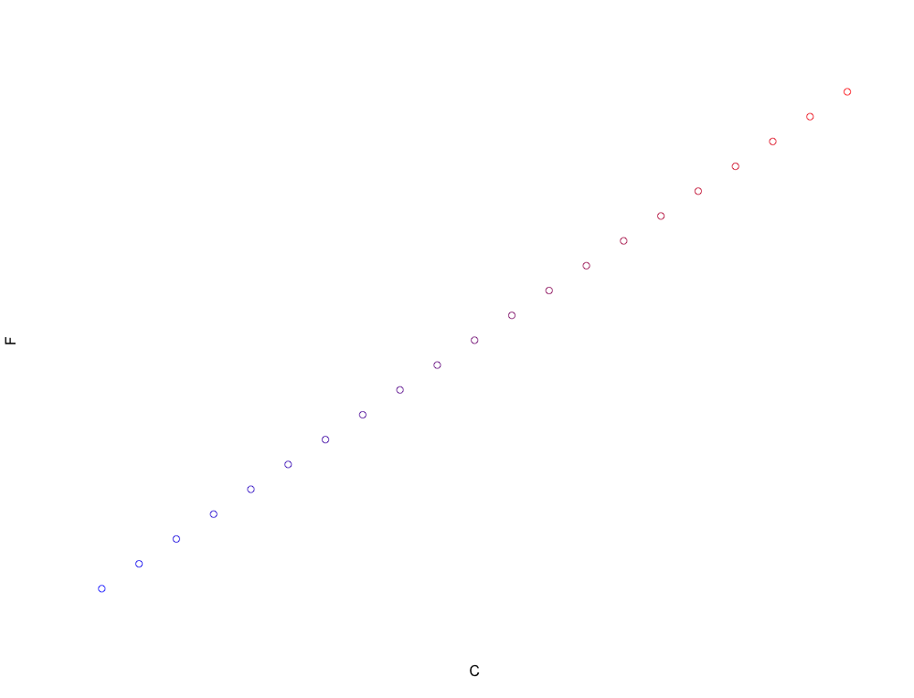
C<-seq(0,100,5)
F<-C*1.8+32
colFunction<-colorRampPalette(c(“blue”,”red”))
plot(C,F,col=colFunction(21))


Learning R, part II: Importing Data

Rplot2

R is often described as having a particularly steep learning curve, and to some degree that is true. However, one of the steepest parts of this learning curve, at least for me, was the simple task of pulling in existing data.

In the last post, I told you to use RStudio, and that advice still holds. Bringing in files and importing data may be the place where RStudio has the largest impact on lessening the R learning curve.

In fact, pulling in data to vanilla R (vanilla in this context is simply some software without any add-ons or extras; in this case the standalone build of R) is something that I don’t actually know how to do off the top of my head. I know that there’s a get something something command, and I could probably figure it out easily by searching for it (this is also a skill you’ll pick up quickly using R), but for a number of reasons I don’t have to.

First and foremost, you shouldn’t feel bad or embarrassed if you forget a command like this. I could go to any search engine and type ‘importing data to R’ and I’m going to get…about 36 million hits. That knowledge is out there. If I need it, I can find it.

If I’m using RStudio, though, I have other options. Now, there are specific cases where you might want to write code to pull in a file so that you don’t have to stop and do it by hand, but for the most part you’ll likely just be pulling in one file at a time.

Let’s start with a file from whatever spreadsheet program you choose to work with. I’ve entered in some quick numbers into a file, to demonstrate:

You can see that I’ve used the first row to toss in some variable names, though they’re not super descriptive. If these variables had any sort of meaning I could have put those names in the first row, and R will read them. It is also perfectly fine if you don’t have variable names in your file, R will take care of that for you.

Once you have this file, you’ll want to save it as a CSV file in a place where you’ll remember it. You can name the file whatever you want, as you’ll have an opportunity in our next step to change that name for the purposes of R.

In RStudio, on the Environment window, there is a button marked ‘Import Dataset.’ Click it, and you’ll get a file dialog window that you can use to find your file. Once you have that selected you’ll be taken to another window that you can use to specify characteristics of your file. This window looks like this:

There are a number of important components here. First off, ‘test’ is what I named my CSV file. If I wanted to call this dataset something different in R, this is where I would change it. I’m going to go with ‘dataExample1’ for my data, but feel free to choose whatever name you’d like for your own.

The section in the upper right is showing what the values in my file look like at the moment. You can see that the values are in fact comma separated (that’s what the C and S stand for), and you can see that ‘Comma’ is correctly selected in the ‘Separator’ box. If you have other delimiters you can change this value now.

In the lower right you can get a feel for how this file is going to look once it is in R. You may notice two rows of variable names here (don’t be too confused by the fact that I used, in my file, names that are redundant with R’s default names). The bold row at the top are variable names that R has generated for this file. The set below are those from the CSV, because R thinks they are values at the moment!

We can easily fix that by choosing ‘yes’ for heading instead of the default ‘no.’ This should remove that second set of values and take your own variable names into the bold area. If you didn’t come up with your own variable names you can leave the heading selection alone.

You may at some point need to change the values for Decimal, Quote, and/or na.strings, but it is unlikely you’ll need to do this early on. For now, don’t worry about them unless you know something different about the values in your file (such as commas used as decimals).

For reference, I’m left with something like this:

Now, click ‘Import,’ and your data should be pulled into R and named with whatever name you assigned in this window. If things have worked, you should see this name show up in your Environment window. This file is now present in the global Environment, and we can write code that references it just like we wrote calculations that referenced x and y last time.

You might be thinking, ‘that was easy.’

Well, yeah. It kind of is.

You’re certainly going to run into more complex problems as you start to pull in larger and more complex datasets, but if you understand the core of what we just did above you understand the most of it. The main trick is getting your data into a clean and orderly CSV file.

We will focus next time on some of the things you can do with R now that you have a dataset in the Environment, but it’s probably worth giving you a bit of a few of these this time, just to give a feeling of what’s coming.

Again, I named my dataset ‘dataExample1,’ so change that value to whatever you named your file and then try running the following code:

summary(dataExample1)

cor(dataExample1)

Those should be pretty straightforward, but in in the spirit of giving you something complex, feel free to try this, as well:

image(c(seq(1,nrow(dataExample1),1)),c(seq(1,ncol(dataExample1),1)),matrix(unlist(dataExample1),nrow(dataExample1),ncol(dataExample1)),axes=FALSE,ann=FALSE)

It should work, as long as you’ve input a CSV file with all numbers, without missing values. If it’s not working for you, see if you can’t fix it.

I also tend to use more code than necessary, so also feel free to suggest improvements that would do the same thing!

Learning R, part I: Getting started with R

rplot1

There are many posts, articles, books, and other resources out there that can teach you how to use the software package R. The goal of this series of posts is more or less to do the same: to give you enough of an understanding of R that you can begin to use it, and even start to learn how to use it on your own.

I am hardly an R expert. The point is that you don’t need to be an expert to use R in very meaningful and useful ways. The goal of this first post is to give a big-picture idea of what R can do, and get you over the first few major stumbles that you are likely to encounter.

It seems obligatory in any R tutorial to first point you to the place where you can download R, which is here:

https://cran.r-project.org/

CRAN stands for the Comprehensive R Archive Network, and you’ll see it come up a lot. For now you simply need to choose your operating system and then download the file appropriate to run programs on that operating system.

Put away your wallet; R is free. That’s kind of one of the big pros.

Now, if you open R for the first time you’re going to be treated to something that looks quite a bit like this:

I am here to reassure you. You may be intimidated by this, and that is perfectly fine. This may very well be the first time you have encountered a command line interface. That is okay. You may be searching for other things you need to do right now instead of learning R, or deciding whether you want to just maybe worry about this tomorrow. Stick with me; today is the day.

What you are seeing is more or less the core of R. You can type things in the command line, like 3+4, and R will provide you with an answer (hopefully, 7). If you want, this is a reasonable time to type in some calculations, and to see that R is just like your calculator from high school. Play around.

If you’re still feeling anxious about typing into a command line, don’t worry. While you are probably always going to have to type things to use R, there are a number of better ways to go about it. In fact, one of the main things I want to get across in this post is fairly simple:

If you want to instantly be better at using R, use RStudio (or something like it). 

RStudio is simply a program that keeps track of all the information that you are feeding in, storing, and pulling out of R. It still uses the core of R we saw above, and that is why you need to install R first in order for RStudio to do anything.

You can download RStudio here:

https://www.rstudio.com/

The good news is that RStudio is also free. You may notice that there is a choice for commercial licensing, but that is only if you work for a company that can’t work with AGPL-3 licenses. The AGPL-3 is one of the same licenses that R uses, so if you are running R then the non-commercial free version of RStudio is no different, at least from a licensing and cost standpoint.

The first time you open RStudio it should look something like this:

You may notice that you still have a command line over on the left (more appropriately identified as the Console by RStudio), but may find some solace in the added Environment/History and Files/Plots/Packages/Help/Viewer windows off to the right. The console works just like R did, and you can type 3+4 the same as you did before.

Again, RStudio is just running an instance of R here. Above and beyond this, though, it is also keeping track of a lot of things that you’d otherwise have to track on your own in other programs. That’s what’s in the windows on the right, but we can make it even better.

Go to ‘File’->’New File’->’R Script’

This will pull up another window in the upper left, pushing down the console to only a quarter of the screen (take that, Console!).

Think of this new script window as a text document, like a Word file. You can type things in here, without the worry of being on the command line. You can run sections of this document, or all of it at once.

Try typing 3+4 again, this time into the script file, then highlight it and hit ‘run’ (or use your operating system specific hotkey, usually some variant of CRTL+Enter). The selected code is taken down to the Console and executed, producing the same answer as before.

Unlike before, we can store a number of lines in our script document and run them all at once, or any number of them at a time.  Try typing out some other calculations, each on their own line in the script file. Highlight them all, and then hit run again.

You can see that each of my calculations were executed in sequence, giving the answers of 7, -1, 0.75, and 12 to the statements of 3+4, 3-4, 3/4, and 3*4.

I should say, you’re not just limited to simple computations. We could type something much more complicated, and R would handle it and give an answer. We will get there.

Now, you might have noticed that the Environment window has stayed empty during the calculations you have run so far (assuming you haven’t jumped ahead ^_^). The reason for this is that we have just been doing one-off computations the same as you might on a physical calculator. Nothing is being stored, so the environment remains empty.

Try typing the following into the script window, then highlight and run it:

x<-3
y<-4
x+y

You should see these lines executed in the console, and you should see some information pop up in the Environment window. The lines x<-3 and y<-4 should have printed and executed in the console, but without producing an answer. That is because they weren’t computations, but rather variable assignments. By giving a variable name, pointing an arrow at it, and then giving some value we want to store in that variable, well, we store that value in that variable.

The final line should have done the same as typing 3+4; that is, it should have returned the answer 7. You also might have noticed that x and y showed up in the Environment window, letting you know that these are persistent assignments that can be used in other computations. Try typing x+10, and you’ll get an answer based on the x that is being stored in this environment. If we hadn’t stored an x you would get an error:

Error: object ‘x’ not found

Now, if using x and y just gave you flashbacks to grade school algebra, take note that there’s nothing crazy going on here (yet), and there’s nothing special about x and/or y. Try typing:

cat<-3
keyboard<-4
cat+keyboard

While you might not expect that cat+keyboard=7, hopefully you can start to see how this makes sense given what we have given R to work with.

We also aren’t limited to only storing things on a one-to-one basis. We can use the combine function to combine a number of values into a set. Try typing:

number<-c(8,6,7,5,3,0,9)

You should see this new variable ‘number’ come up in the Environment window. The [1:7] simply means that the values are stored in this vector in locations 1 through 7. We can use this information, later, to call specific values from such vectors and lists.

Now that we have these values stored in ‘number’ we can do computations to them just as we did to x and y, earlier. Try typing the following:

number+3

Our answer should be the same length as our ‘number’ vector (that is, length 7). When we tell R to take ‘number’ + 3, R (correctly) interprets this as each value of the vector number plus 3. Thus, it performs the calculations:

8+3
6+3
7+3
5+3
3+3
0+3
9+3

Take note, this does not change the values stored in ‘number’ because we haven’t done anything to change them. We’ve simply executed a one-off computation using them.

We can also graphically display the information stored in ‘number’ with a simple histogram, by typing:

hist(number)

Now, try the following:

number+number-number
number*number
number/number
number+number[5]

Think through these commands, and see if you can figure out the calculations behind each of the answers. If you understand what’s going on here you understand a good portion of R.

If you’re feeling particularly good about what you’ve done so far, you can also try typing:

plot(number, number*number)

To some large degree, it’s really as simple as that.

Now, if you want to see something more interesting, try typing:

plot(number,number,type=”steps”,col=”blue”,xaxt=’n’,yaxt=’n’,ann=FALSE)

You don’t need to figure out what’s going on in that plot yet, but you might have fun giving it a try.

Before we finish, I should say that you can save your script files and then come back to them whenever you want. You can have multiple scripts open at once, and have them all working on the same Environment (we can deal with local and global environments much later). You can also save everything that’s going on in the Environment as the workspace of a project, so that your work is easy to come back to right where you left off.

Congrats, you’re using R!