Paul G Curran

Hi everyone – today we’re going to talk about Kickstarter.  We’re going to talk about Kickstarter because I’m currently Kickstarting a Kickstarter project related to the blog.  Kickstarter.

I talked about Tetris a few weeks ago (here), and examined the counts of pieces across a number of games. That got me thinking about Tetris pieces, especially when I started to look at some of the Tetris variants that people have programmed.

One of the things that lingered in my mind was the idea that all Tetris pieces are made up of four 1×1 blocks.  I’ve played some variants over the years (many of them official) that did some other things with these four blocks, like allow for corner-to-corner connection (unacceptable!) instead of strict face-to-face connection, but none to my recollection that changed the standard use of four 1×1 blocks per piece.

So what would happen if we changed around this simple building block (haha) of the Tetris franchise?

The simplest Tetris game would be a situation where each piece was made from one 1×1 block.  When I say simplest, I’m not sure I can express that enough.  You just get the same piece over and over, and try to build lines with it.  It’s basically two-dimensional Minecraft where the pieces fall from the top and sometimes disappear.

The two 1×1 block case is hardly different, actually.  There’s still just one piece, though at least now rotation matters in game.  Not that much, though.

The three 1×1 block situation starts to get a little more interesting.

You still only end up with two distinct pieces – a hooked piece and a straight piece.  It might actually make for a fairly interesting (if not somewhat simpler) game.  Tetris Jr., perhaps.  Someone code this.

A situation with four 1×1 blocks is the Tetris we know and love, and produces seven pieces.

You should be familiar with these, but you can also see that they’re basically just an extension of the pieces in the three 1×1 situation.  You can add a 1×1 block to the first piece (in the three 1×1 case) to make the square (O) block.  You can also add a 1×1 block to that piece to make the S, Z, J and L pieces.  You can make the T out of any of the pieces, but the only way to make the straight (I) piece is to add on to the straight piece from the prior set.  It’s a rather simple but interesting point.

So we already have a pretty interesting set of numbers here.  The first two cases result in a single piece, then we move to two, then to seven.  We’re more than doubling with the addition of one more 1×1 block because each piece already able to be made can produce a number of new pieces.  The more complex those pieces, the more places a block is likely to produce a new unique piece when placed.

Let’s see if we can build a set of Tetris pieces with 5 1×1 blocks.  By that I mean, I’m going to spend some time doing that in Excel, and the next thing you’ll see is that completed.

So there you go.  That might have seemed quick for you, right?

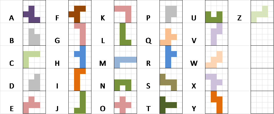
I worked each piece separately to make sure I was covering all bases, and didn’t create duplicates within the same base piece (from the four 1×1 level).  I shaded pieces red if they duplicated a piece already made by a previous base piece.  That leaves us with 18 unique pieces, which we can see a bit clearer in this picture.

There you go.  Someone, make this game.

There are two things that stand out to me.

First off, there’s a lot more pieces, but still only one straight piece.  Since it simply is what it is (all the 1×1 blocks you have to work with, in a line), there’s only ever going to be one while the rest of the pieces keep expanding.  If you thought you were waiting a long time for a straight piece in the four 1×1 version you’d hate a version like this.

You could look at it this way:

That’s only going to get worse, though I’m not going to go past five 1×1 blocks given how much more work the six 1×1 case is going to be.

The second thing that stands out to me, though, is how close some of these pieces look to actual letters.  There are also 18 of them, and while some of the duplicates fail the rotation test in Tetris, they would look distinct enough on paper.

In fact, we’d only need eight reflections to get up to 26, which is a pretty interesting number because at that point we can build a substitution cipher with the English language.  So…let’s do that.

I didn’t really expect to end up with a substitution cipher when I started this post, but I suppose time makes fools of us all.

The nice thing about this is that each letter can fit in a 4×4 square, allowing for even further ciphering by expressing those letters not as letters but as a string of numbers.  Off the top of my head you could easily do that one of two ways.

The first would be expressing a letter as a string of numbers based on which squares were filled in.  In that way, ‘a’ would be 6/9/10/14/15, or 69101415.  The information can be parsed out without explicit spacing due to the lack of any letters in the cipher using the ‘1’ square.  If there’s a 1 in the number it means that it – and the next number following – are part of a two digit number.  In that way you can easily break 69101415 into 6, 9, 10, 14, 15.

The numbers also don’t need to be in order, so the letter would be just as preserved written as 10149156.

Each letter could also be written as a 16 digit binary number (realistically less if we figured out which squares were never used).  In that way, ‘a’ would be 0000010011000110.  If you read my post on binary math you know we could easily translate that number into base 10 and come up with 1,222.

I think I’ll revisit this one in a few weeks, as I think there’s some other stuff we could do with this.  For now, though:

A few weeks ago, Zane Lamprey broke the Guinness Book of World Records record for “Longest live audio broadcast streamed over the internet” with 25 hours of non-stop broadcasting.  He also successfully funded his new show “Chug” through kickstarter, for those of you who ever saw his prior shows.

During this 25 hours Zane and his co-hosts and guests talked about a lot of stuff.  There was a limit of 5 seconds of continuous dead air, so they pretty much talked non-stop (especially Zane after learning about the 5 second rule).  One of the things they talked about was the idea that while coin flips are basically fair, coin spins tend to be a bit more biased.  Allegedly, it’s even worse if you stand a coin on its edge and then bump the surface on which it’s standing.

The general idea is that a coin flipped with enough velocity imparted into rotation is basically fair.  A coin flipped by someone looking to bias it may be able to shift that fairness slightly, and someone looking to professionally bias it for a living may be able to eradicate that fairness altogether.  Practically speaking, however, if you’re trying to flip a coin in a fair way it’s pretty easy to do so (e.g. get a good toss and spin on it, and don’t pay attention to which side started up or down, or better yet have someone who hasn’t seen this call it, etc).

Things happen differently when you stand a coin on its edge and then agitate the surface, or spin the coin instead of flipping it.  In both cases it is alleged that you’ll see a lot more ‘tails’ results, at least on Lincoln Memorial pennies.

The bottom line is that a coin flip or spin is simply a system of knowable physical properties.  A physicist with enough gumption (these folks are mathematicians) could sit down and write a Lagrangian for the system to determine the outcome given starting conditions (e.g. position, initial velocity, initial height, etc).  I’m by no means saying that it would be easy, I’m just saying that it could be done.  [The easiest case to start on – those of you who have already opened their lab notebooks – might be the standing on edge case where the force comes from one side.]

Without such a Lagrangian, people like to just come up with reasons for things they observe, and then apply them without worrying about pesky things like the scientific method.

For instance, people who have examined this so far have come up with two main suggestions, the first far dominant over the second.

1) One side of the coin is heavier than the other, and so a spinning (or disturbed standing) coin will fall toward that side.  Thus, the other side will come up more often.

2) The way coins are struck leaves the edges to one side smoother than the other, and so a spinning (or disturbed standing) coin will fall toward that side.  Thus, the other side will come up more often.

Both would appear to make some sense, though warrant further examination.

Now, I’m also not saying that it’s by any means practical to deduce any of these smaller effects by brute force statistics.  The whole point – as will hopefully become apparent – is that by manipulating these effects we can potentially make them large enough to overpower any potential smaller confounds (like imperfect spinning, or the fact that the table I’m spinning on isn’t a polished, frictionless surface).  There is a balance to be struck here between the extremes of dismissing an experiment out of hand because it would be impossible (or impractical) to do it perfectly and not doing an experiment at all because you think you know how things work and don’t want to take the time.

Let’s start with some coin flipping.

Most of this research on pennies is a few years old, and as such focused on the old US penny design with the Lincoln Memorial on the ‘tails’ side.  I was able to find one of those in excellent condition sitting around – the idea being that a penny that had some wear might a) collect ‘gunk’ on one side or the other, leading to an unequal weight distribution, b) receive uneven wear on the faces of the coin, leading to an unequal weight distribution, or c) receive wear on the edges, removing any bias in edges from striking.

Flipping was rather boring, and led to a fairly predictable outcome.  Of 50 attempts, 24 came up tails and 26 came up heads.  Is that biased?

Well, I could write a much longer post just about how many times you realistically have to flip a coin to tell if it’s actually biased, but let’s just quickly compare this result to something which we have reason to believe should be quite a bit less biased.

If you read the post a few weeks ago you know how to generate random numbers in a program like Excel or Google Docs.  We can quickly generate 50 random numbers that way, which will fall between 0 and 1.  Then we can check what proportion of those fall into the top or bottom half of that scale.

I would suggest you do this for yourself just to see how such a random distribution breaks down at this sample size.  My first draw got me a distribution of 23 ‘bottom’ and 27 ‘top’.  It’s perfect to illustrate my point, so I’ll stop there – 24/26 split on coin toss seems fair enough to me for all practical purposes.  I could flip it again until I have the same number for each side and then stop there – would that satisfy randomness any better?

No, that would be cheating.

How does this same coin fair on the spin test, though?  Well, it’s a little worse.  This time the split is 29 tails to 21 heads.  I’m a little more impressed with this, for two reasons.

First off, it’s a little more outside the range of what I’d be expecting.  You might say, well you just observed a 27/23 split on something you are holding up as random, so why is two more off this that impressive?

Well, second (off?), we have directionality in our hypothesis this time.  The expectation is that tails will come up more, which is what is happening.  I’m confirming something that has already been shown, rather than deriving something from sheer exploration.  When flipping I wasn’t expecting a bias in one way or the other, so being convinced of a bias in either direction should be more difficult.  How much more difficult is an entirely different discussion.

It should be said that these spins – at this point and continuing through the rest of this post – have all been done with the same direction of rotation relative to the ground.  That direction is clockwise looking down from above, or a right-hand rule result of negative Z in a Cartesian coordinate system.  There is much to be said about testing a counterclockwise or positive Z spin, but that’s more than I want to realistically talk about today.

I wondered if this would hold up on other coins, so I found another shiny new penny – but this time of the new ‘shield’ penny variety.  Without a hypothesis here I’m back to a bit of exploration, but found similar results of 29/21.  Interestingly, though, this time in favor of heads instead of tails.

By the way, I have no reason to believe that this or any other coins I have is biased in flips (and frankly, I simply don’t care), so I didn’t check flips on this or any other coins.  Looking back I’m wondering why I even did on the first penny.

Anyway, looking at one type of penny at a time seems prudent as a start, so I’m simply going to let the shield penny slide for now.

There’s another part to this, though, and it’s the whole standing up and bumping.  The idea is that if you put a penny on its edge, then destabilize it, it’s biased again toward tails.

Turns out it’s not the easiest thing to stand a penny on its edge, but the results seemed so clear so quick that I didn’t have to do it for long.  Of ten attempts, I ended up with 9 tails and only 1 heads.

Before you start speculating, I also tried to vary things as much as possible (you might say introduce as many confounds as possible) as to check that it wasn’t just the fact that my table was tilted in one direction or another.  If one trial was in one area I tested the next with the coin 180 degrees from that, then 90, then 180 from the 90, then a whole different area of the table.

I also tried to bump the table with fairly uniform strikes from my fists some distance away from the coin and from random (and sometimes dual and competing) directions.  Nothing really seemed to change the fact that this coin wanted to go tails up.

Intrigued, I reached the part where science comes into play.

Some of the brightest people I’ve ever worked with have always pushed the idea that unless you’re able to manipulate an event, you don’t actually understand it.

In this case, people claim to understand how this whole penny problem is working out.  They postulate that it’s one of the two above ideas, but I’ve been unable to find anyone who has actually sat down to manipulate either of them to actually strengthen (or weaken) the effect.

So, I sat down to try and strengthen (or weaken) the effect.

The first thing on my mind was how to see if weight played any role.  There are two obvious ways to manipulate this – add weight to one side or remove weight from the other.

Not wanting to deface any coins at the moment, I decided to try to add weight to one side of the penny by simply adding some small cut squares of packing tape.  I made sure that they didn’t extend to the edges so that they wouldn’t interfere with any spinning, and the result was a coin that from a distance didn’t really look much different than normal (since packing tape is transparent).

I put the tape on the tails side to see if I couldn’t negate the effect that we’re seeing.  If the heads side is in fact heavier, then adding weight to the tails side should (at some level of weight addition) eliminate that bias.

Ten trials with the coin stood on edge, and no great change in which way they fell.  Instead of 9 tails and 1 heads, this time I found 8 tails and 2 heads.  The difference is in the direction I was expecting, but it is by no means the game-changer that would eliminate that bias.  Wondering if the weight was enough to do anything, I decided to try the same with spins.

Keep in mind, the last time I tried spinning this same penny resulted in the expected bias toward the tails side:  29 tails vs 21 heads.  The effect wasn’t as strong as the standing on side effect, but it was there.

Of 25 spins (I was getting a little lazy), the effect does seem to be reversing.  By putting a small amount of tape on the tails side of the coin, it now appears to be biased a bit toward falling heads up – 16 heads to only 9 tails.

Putting the tape on the other side of the coin is also biased toward heads, though.  It’s a little less, 14 vs 11, but it might mean that the tape isn’t really enough to do much, or there’s something being canceled out here that’s bringing things back to near-random.

A little bit of tape is one thing, but I found myself wanting to really knock this thing out of the park and fully bias a coin in one direction or another.  Frankly, a penny is too small to add much weight to, but a quarter gives a lot more surface area to play around with.

To start I figured I’d check to see if an old (but good quality) eagle-backed US quarter would be biased in the spin test.

Emphatically yes, it would appear.  In the first 10 spins only 1 came up heads.  I tried another quarter, and it appeared to be similar.  I could test more quarters and see if there’s a consistent effect here, but what I’m really trying to do at this point is simply show that something I do can change the result.  I don’t care what the starting result is so much as I care that by some intervention it can be changed.

That intervention is (ostensibly) weight.  A few pieces of tape on a penny is one thing, but for this test I wanted to really just overpower smaller effects.  So, I used some tape to carefully tape a dime to one side of the quarter.

For reference, I used the old loop tape onto itself and put under technique, like you might use to hang a poster on your wall.  That way I didn’t run the risk of taping too close to an edge and introducing other variables.  The dime sat safely in the middle of the face of the quarter, so there was no worry that its edge might graze the table either – if the dime was touching the table it was already well on its way to (read: unavoidably) falling onto that side.

The weight of a dime would seem to be drastically greater than the weight differential of either side of the coin,  and my only concern was the fact that I’d done something aerodynamically detrimental.  Something to think about, though it turns out (later) that other things might actually be at play.

[By the way – as a quick aside – the addition of this weight was enough that the quarter was no longer willing to stand on its edge, thus making the standing and bumping aspect of this impossible.]

If the above weight arguments are working properly, then the idea would be that the head side of this quarter was heavier, and thus causing the quarter to fall with the tails side up.  The first natural thing to try, then, was to place this dime on the tails side to see if that weight would pull that side down faster, leaving the heads side up.

And this is where things start to get weird.

10 spins.

10 tails side (with dime taped to it) up.

Oddly, then, it would seem that I’d solidified the effect that had already been occurring.  There is simply no way that the weight differential was still in favor of the heads side of the quarter (if it ever had been).

There’s a simple way to confirm that – move the dime to the heads side of the quarter and see if that will reverse the effect.

Well, yes.  10 spins, this time 8 heads (with dime up) and only 2 tails (with dime down).

I was such in doubt of my own results that I ran both cases again.

The dime on heads side was similar, with 7 heads (with dime up) and 3 tails (with dime down). 

I kept spinning the dime-on-tails-side hoping that I’d eventually get a heads (dime side down) result.  I have yet to reach that point.  I spun 40 more times, just to get to a nice even 50 overall, and have yet to end with anything other than a tails (dime up) result. 

It only took me a few spins on this second run to figure out what I believe might be going on in this case, though.  It’s not the fact that a heavier side will fall (as it might be if it was standing on edge), but rather that introducing more weight on one side of the coin shifts the center of mass.

Why is the center of mass of the two-coin system important?  Well, it’s potentially important on the one-coin system as well, but in the two-coin system it has a pretty profound impact on axial tilt even on a pretty hard spin.  Systems rotate around their center of mass, so if that is pushed outside of one of the faces of the coin (or toward one of the faces, in a less extreme example), the axis will drift to keep that side inside the spin. 

That is to say that even on a spin with a whole lot of energy the spinning coin fails to achieve a spin perfectly perpendicular to the surface on which it is spinning.  It maintains an axial tilt that keeps the dime side ‘internal’, so to speak.  As the coin slows, the axial tilt increases, as it’s only the energy in the spin that is keeping it even close to a zero tilt system.

The short answer (and longer question) is that an unequal distribution of weight might cause differential effects in spinning vs standing coins due to the fact that axial forces can come into play during a spin but only gravitational forces will come into play (ideally) in a standing bump test.  

All in all, from a numbers point there seems to be something here – though it’s certainly not as simple as it might first appear.

What can we really get out of this so far?

Well, edging of the coin might not be a strong factor, at least not as strong as some of these weight changes.

The bump test and spin test seem to be producing effects of different sizes, or at least effects that are more robust to interference.  More importantly the bump test might be driven by gravity and the spin test driven by shift in center of mass.

Placing a relatively large weight on one side of a quarter tends to favor that side ending up face up, though there are also some problems of shift in the center of mass and axial tilt.  This might come into play in all coins, to a lesser degree. 

Overall, though, I think I’m left with more questions than answers.

There may be reason to believe that at least some of the forces that might be working on a spinning coin are based on spin direction – I’ve kept that constant so far but might find drastically different things with a reversed spin.  The only thing that should operate this way would be the Coriolis force, which seems like it may be one of the smaller effects operating in this system.

Taping a dime to a quarter is a quick proof of concept, but the additional protrusion that this introduces leaves me a little unhappy.  I’d like to figure out a way to increase the weight distribution without changing the shape of the coin, but that would seem to involve some metalworking.  

I didn’t look specifically at edging yet, but it would seem that a quick brush with some sandpaper might be enough to give one edge or another a smoother…edge.  The problem with this is – unlike some tape on the face of the coin – that such a technique is destructive to the object being tested.  Unless I had two coins that I believed to be – for all intents and purposes – identical, I couldn’t test the second edge sanded alone after I’d already sanded and tested the first one.

All in all I thought this was going to be fairly straightforward, but some of these odd results have be a bit intrigued.  I’ve put a (Part I) on this because I want to spend some time thinking about this as well as running it past others – by all means if you have suggestions or thoughts post them in the comments.  I’d love to figure out what’s actually at play here.

It’s Stanley Cup Finals time, and that means it is time to look at some hockey numbers.

(borrowed from http://www.printactivities.com/Mazes/Shape_Mazes/stanley-cup-hockey-maze.html in the spirit of fair use)

I always say that for most sports I don’t care as much about win or lose as much as I care about just seeing a good game of [sport].  I think that holds fairly well for hockey, though in this particular Stanley Cup series I’m cheering pretty hard for my hometown team (the Blackhawks).

Nothing says good game of sport like playing it longer than normal, right?  A blowout in either direction is usually pretty boring, and coming to the end of regulation in a tie usually means just the opposite – a fierce, well-matched game of sport has likely been played to that point.

If you like watching hockey, you’ve already received a sort of buy two-get one free deal on the first two games of the Stanley Cup Finals between the Blackhawks and the Bruins (and Bruins fans got an extra freebie on that third game).  Two full periods – and some change from two other partial periods – were played outside of regulation in just the first two games.

If you watched those games, but don’t really follow hockey a lot, you might have been scratching your head at some point during the second or third overtime.  “When do they get to the point where it’s like in the movies and guys just shoot on the goalie?”

Well, we’re in playoffs now, so…never.

You see, the rules of overtime play are different in regular season and post-season play.  In regular season hockey, overtime is a sudden-death (i.e. first team to score wins) five minute period, followed by a short break and then a shootout.  In post-season play, you just keep playing sudden-death (but otherwise normal) 20 minute periods until someone scores.

As long as no one scores, the game will simply go on and on.  If you’re interested, the longest game of NHL hockey extended into the 6th overtime, and finished with a total of 176 minutes and 30 seconds of ice time.  The game was in 1936 between Detroit and Montreal, and the goal scored 176 minutes into the game was the only goal of the game.  If I could go back in time and watch any one game of hockey, that might just be it.

You may be asking “Yeah, but why make them play so much hockey?  Why not just go to a shootout?  If it’s good enough for the regular season it’s good enough for playoffs.  Come on.”

Well, truth be told, shootouts aren’t really good enough for the regular season.  It would appear that they’re tolerated simply because they make great ends of movies (i.e. they’re fun to watch).

I’d always been told that the reason shootouts aren’t in the playoffs is because they are poor predictors of actual skill.  Granted, they measure a particular level of skill (I couldn’t go out there and score a shootout goal against…well, probably anyone), but they completely fail to differentiate skill levels within the range of skill being measured (professional hockey players).

Imagine if a basketball game tied after a few minutes of overtime simply came down to a free throw competition, or – more appropriately – a series of one-on-one layup attempts against a team’s best defensive player.

Imagine if a baseball game’s extra innings consisted of every fielder except the pitcher and catcher taking the bench, and every hit simply being an in-the-park home run (actually, that might be awesome).

Imagine if football’s overtime was, well, exactly as they do it now.  Come on, it’s not like they want to play extra football.

Anyway, I’ve always just accepted the notion that this skepticism surrounding shootouts was true.  Given the shortened season this year, though, I figured it would be easy enough to go into the team records and pull some data on who actually does win the shootouts in the regular season.

Given that teams play each other (duh), I was able to cover a large majority of the shootouts that took place this year by looking at three random teams in each division (there are five teams in each division, three divisions in each of two conferences).

This sample produced 83 regular season games which were decided by shootout.

I was also able to determine – based on their standings at the time of the game involving the shootout – which team was favored to win, and which was the underdog.

If shootouts are actually getting at the skill of the team, then we’d expect to see teams with better records more likely to win shootouts (because they’ve shown themselves to be better at winning games, which is the main established criteria of hockey skill).

I’m not sure I really have any way to continue to hold you in suspense other than this sentence, so here is this sentence that’s really just designed to hold you in suspense for the time it takes you to read it.

Of those 83 games, 45 (54.2%) of them were won by the underdog.  Only 38 (45.8%) were won by the team with the better record at the time.

Now, that’s not too far from random chance (a 50-50 split), but random chance isn’t what we’re going for here.  Random chance would be if the NHL simply ended ties in regulation with a coin flip.  If we wanted to show that shootouts are useful they would need to display some bias toward the team with the better record.

Not only are we not seeing a bias toward the winning team, we’re potentially seeing a bias against them.

So next time you’re watching a shootout in regular season play (or someone you’re with complains about lack of shootouts in the playoffs), take a coin out and give it a flip beforehand.  It might actually be a little bit more fair.

My birthday was this week, as were a number of my friends’ birthdays.  I’ve always held the belief that the week or two surrounding my birthday is heavily populated by other birthdays of people I know, more so than any other time of year.  I know a few people that share my birthday, a few people that are the day before, a few that are the week after and before.

It can’t be that my birthday week or two is special, though, right?

facebook is only good at a few things, and holding on to birthdays is one of them.  If you go into the events sidebar and then click on some stuff that makes sense when you see it you can eventually get to a calendar view listing off all your friends’ birthdays (or at least those that use facebook and have put their birthday on it, and that are telling the truth).

It’s a pretty easy way to pull down some data on a large majority of my friends’ birthdays.  I have no reason to believe that birthday would have anything to do with friends’ refusal to use facebook, so hopefully that data is missing at random.

It’s a fun exercise, and I’d recommend you to do it if you’re bored one day.  You might also think that your time of the year is special, and – well – if you do I’m here to tell you that it’s probably not.

Well, unless your birthday is Halloween:

October 31st seems to be the most popular birthday, by a decent margin.  Seven of my facebook friends were born on Halloween (hi guys), with the next most popular date being June 7th (with five people – hi guys).  All other dates have four or less birthdays (hi guys, sorry you’re not popular).

June 7th is pretty close to my birthday, so maybe this is starting to look like I was right all along?

If we’re looking at the days with the most birthdays, we can also take a look at this with the least.  There are a lot of those – days where none of my facebook friends have a birthday.  What’s the longest stretch of birthday-free days?  Well, there are two stretches of five birthday-free days.

Interestingly, they are right around the last place I would have expected them.

Well, that would seem to fly in the face of early June being anything particularly special.

There’s still some other things we can look at, though.  How about months?  What’s the most popular birthday month?

Oh, months have different numbers of days?  Okay, here’s the same thing but normalized.

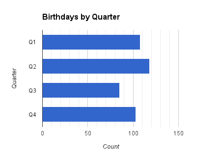
Or we could just look at quarters.

Overall, it looks like the late summer months are somewhat weak, as August and September are the only months where the average birthdays per day drops below 1.  Interestingly, May/June – despite some large gaps that we saw earlier – is still quite strong.  Both these months are closing in on one and a half birthdays a day.  This might actually start to explain some of what I’ve been picking up on through the years.

Perhaps the fact that June is still such a strong month even with so many days without birthdays is because the days that have birthdays (which happen to be around my birthday) have more birthdays than normal.

Well, the average birthdays per day across the whole year based on my friends’ reported birthdays is right around 1.1 a day.  Those 3s, 4s, and 5s in that above table are starting to look pretty good, right?

In all, it’s kind of hard to say one way or another that any part of the year seems to be the most populated (though late summer does sort of seem to be kind of desolate).  It is certainly clear that I have been a least a little biased by remembering the birthdays of individuals near mine (probably because I say at least once “hey your birthday is pretty close to mine!).   The spread of other birthdays does seem to be decently random, though Halloween still seems at least a little confusing.  What’s the deal with Halloween, seriously?

Vampire/werewolf/zombie/ghost doctor conspiracy?

The moral is clearly that you should never trust anyone with a Halloween birthday (sorry guys – you might be ghost doctors or something).  Happy (belated/eventual) birthday, everyone!

Time for some more TPIR.  Today, we’re going to talk about Contestants’ Row again.  If you missed the first post on Contestants’ Row you might start here, though unlike some posts this one is fairly standalone.

I’ve been coding more episodes, and one thing that has started to stand out is the proportion of time that the contestant who has the last bid on Contestants’ Row wins.  It is not surprising that they would win the bidding most frequently, though it seems that they win a lot.

From a simple betting standpoint they should have the odds in their favor for two reasons.  First, they get to choose a bid mapping to a range of numbers with full knowledge of the other contestants’ bids.  Second, no other contestant gets to bid after them, and thus no other contestant has the potential of cutting out a part of that range of numbers.

For instance, if there are bids of 600 and 900 registered, and a contestant bids 601, they now have the range of numbers from 601-899 covered.  If it is the third contestant bidding 601 there is still another contestant who could cut that – even all the way down to just one number (by bidding 602 and stealing the numbers from 602-899).  If it is the fourth contestant bidding, that range of numbers (601-899) is perfectly safe.

A simple frequency count on the winner of the Contestants’ Row bids for the episodes I’ve watched reveals that my suspicion is quite correct – the fourth contestant does win a lot.  Like, a lot.

If we break it down to simple odds, the fourth spot on Contestants’ Row has nearly twice as great a chance of winning as the next best spot (39.3% for fourth spot, 21.7% for first spot, 21.4% for second spot, and 17.5% for third spot).

It’s an interesting point that the third position is actually the weakest – they should have some advantage from knowing what the first two bids have been and only differ from the fourth bidder in that they have someone who goes after them.  This may mean that the knowledge of prior bids is simply a much smaller effect than lacking someone going after you.

I have noticed in casual watching that the first contestant also seems to win frequently.  Anecdotally it would appear that they often win by getting exceptionally close to the eventual price, blocking out the other contestants who bid after them.  This would lead to the question: do winners in different positions on Contestants’ Row need to get closer to the price in order to win.

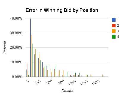
We can take a look at this by looking at the winning bids of each position, when they win.  Particularly, we can look at the error in the winning bids by position.  Because we’re only looking at wins the bias is unidirectional – a winner can’t have bid over the price of the item, only below or exact.

Interestingly, the first position does not has the highest rate of perfect bids (as I might have guessed) – the second position does.  The first position does, however, have the highest proportion of winning bids within a range of $100 – around 45% of winning bids (including those perfect bids and those from $1-100).  In fact, we can rearrange this chart to better illustrate this point.

This shows the cumulative percent of contestants in each position who have won with any given bid or lower. It is clear that when the first position wins on Contestants’ Row they’re actually doing it by bidding fairly well.  The later bidders may suffer from trying to move away from this already established (but good) bid, though that’s hard to identify.

It is also clear that winning from the fourth spot takes the least degree of precision – winning bids from the fourth position are on average off by more than any other position.  This is very likely due to the ability to bid either $1 (securing the range of all numbers below the lowest bid) or $1 above the highest bid (securing the range of numbers higher than the highest bid).  Both these bids have the potential to win while being off by a large margin. 

Because the position moves around based on who wins, a fourth position win actually makes the prior third position the new fourth position.  This is some solace to contestants trapped in the seemingly weakest third position, as long as there are a number of bids left.  A fourth position contestant who loses their bid to the first bidder gets to retain their fourth position – a very fortunate turn of events for them, again given that there are some bids left.

Overall, it would appear that starting in fourth position is the best way to go, though it’s also sort of out of your hands.  While this information might not be practically applicable in the moment, it might make you feel a little better if you get trapped in third position and go home empty handed.

Over the span of my life I have played a lot of Tetris.  I actually just sat down and tried to figure out when I might have reasonably played my first game of Tetris, and let’s just say it was a very long time ago.

I’m not sure I even want to start coming up with a reasonable estimate for the number of hours I’ve played Tetris, because it’s not likely to be best measured in hours (or even days).  I’m sure it would be even worse if we put it into the metric of “if all the [thing] I had done in my life was my full time job, how long would that job last?”  Let’s just say I’m sure I’ve knocked out at least a few 40-hour work weeks.

We’re not here to evaluate my life choices, though, we’re here to talk about Tetris.  Before we continue too far I should also say I’m somewhat of a (Nintendo) Tetris purist.  I’m not going to say that we need to go back to something that will run on a Soviet DVK-2,

But I will say that there’s really no need to go much further than a game that was for all intents perfectly executed to what it needed to be.  To put it in the words of Spock in Wrath of Khan -while lamenting the fact that Kirk allowed himself to be promoted to Admiral out of the role of Captain – “Commanding a starship is your first, best destiny.  Anything else is a waste of material.”

Tetris is meant to be Tetris.  This is Tetris:

Anything else is a waste of material.  Anything else is like bedazzling the Mona Lisa.

Side note, I just thought that up but couldn’t help but google it.  And…someone has actually bedazzled the Mona Lisa.

Anyway, we can talk about Tetris, but if you want a version where you can press a button to quick drop (in Tetris vernacular “hard drop”), or you want to be able to rotate pieces when they’re against the wall and don’t have room (“wall kick”), or you want to see where the piece would be if it were to keep falling where it is (“ghost piece”), or you want to be able to spin pieces to slow their descent (“easy spin” or “infinite spin”), or you want to be able to hold a piece and/or swap a piece into some sort of reserve (“cheating”), well, we’re playing different games.

And you’re playing the one designed for toddlers.  Baby’s first Tetris, perhaps.

Sorry, am I being too hard here?

No.  No, I don’t think so.  But let’s get to the actual point here.

You can see in the above image that Tetris is happy to give you some numbers on what you’re doing.  It’s not really the most efficient to look at these numbers during a game and plan for pieces that might be coming, but it’s interesting to look at after the fact.  “Oh, that’s why I lost – I didn’t get enough square pieces” (said no one ever).

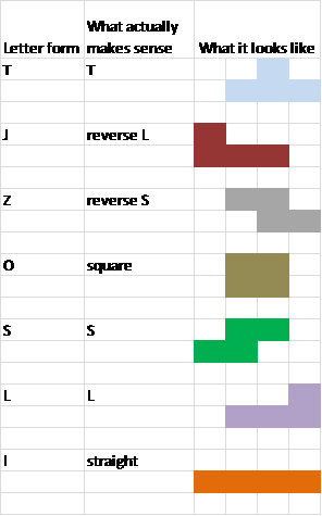
Except we’re really pushing for some Tetris-speak today, so instead of square pieces we’ll call them O pieces.  Yep, that’s their letter-association name.  From top to bottom in the above picture we have T, J, Z, O, S, L, I pieces.

Let’s make it a little easier:

Okay, so now we’re all on the same page.

If you have said anything at the end of the game while looking at the stats, it was probably something relating to your lack (or perceived but unsubstantiated) lack of straight “I” pieces.

Everything I’ve read would tend to indicate that the distribution of Tetris pieces (I’m sorry, “tetrominos“) to be random (if not randomly deterministic).

By the way, don’t mistake that sentence as simple – those are two starts to some pretty deep wiki-spirals.

If the pieces are random, and you play forever (can you play Tetris forever?), you should get roughly a uniform distribution across the types of pieces.  How uniform does uniform really have to be to be considered uniform, though?

I’ve been playing and recording a game or two here and there, but mostly recording the stats from having others play.  All this has produced the following RAW DATA:

From this we can also calculate the proportions of pieces for each game.

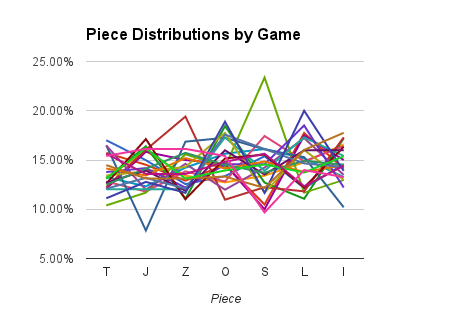
This shows the relative distributions for each game.  Other than one game with way too many S pieces and one game with way too few J pieces, things do seem to be in a fairly tight range.  We can collapse this down to just means to get a feel if this bit of noise cancels out.

We can see that things look fairly uniform, though it’s hard to tell exactly what the expected levels are.  Changing the scaling to bias lets us see what percentage of pieces we can expect above or below the expected uniform distribution per game:

The bias is quite small, and even with these fairly large numbers of pieces (>6700) a chi-square test of association fails to show a deviation from a random distribution.  [ x2 (6) = 9.260, p = 0.16 ]

Oddly, the most common piece in this data seems to be the piece we’re always looking for (the “I”), but this does seem to just be a blip in otherwise random piece distribution.  I guess there’s not really any reason to complain, at least overall, unless I want to complain about having too many of the best piece (and for no reason).

Anyway, why are you still reading this and not playing Tetris?

I seem to have a lot of favorite games on The Price is right, and Rat Race is definitely among them.

I often don’t like games where perfectly skilled play still presents only a chance of winning (like 1/2 Off), but there’s just something about Rat Race.  Maybe it’s the fact that perfectly skilled play always guarantees you at least the smallest prize, or maybe it’s the thought of this guy in the back of the studio diligently applying neon coats to stock rat racers.

For those of you who don’t know the game, it’s fairly simple, but also fairly difficult.

Contestants are shown a series of three prizes, escalating in price.  The first prize is under $10, the second is under $100, and the third is under $500.  The contestant must guess the price of these items within a certain tolerance in order to earn bets on rats in the eventual race.

The tolerance is tied (non-linearly) to the level of the prize that they are guessing.  The first prize must be guessed within $1, the second within $10, and the third within $100.

If the first prize is – for example – $7, then the contestant has to guess between $6 and $8.  Since the error bars extend on either side of the price (it’s not closest without going over like contestants’ row or the showcase), each tolerance is actually only half of the window that the contestant actually gets to cover in terms of range of price.

This also means that completely random guessing (if the prices were completely random, which they’re almost certainly not) would give you a 20% chance of guessing the first item, a 20% chance of guessing the second item, and a 40% chance of guessing the third item.  Realistically, a guess of $350 on the third prize covers a huge part of the likely-to-be-used part of the scale ($250-450), but that’s a question for a different post.

Guessing these prizes within tolerance is at least somewhat skill based, not withstanding that there might be a slight bias toward random luck if played in a smart fashion.  What happens when you have the rats is where skill departs and luck takes over.

You can see that a flawless run of this game leaves you with three rats in the second half of the game.  That second half is the race itself.

Five rats of different colors (yellow, pink, orange, green, blue) race on an S-shaped track (it’s actually $-shaped) that gives them each an equal distance to cover.  Not unlike horse racing, the contestant is trying to pick both the rat that wins as well as those that place.

The game is often played for a car, or something else fairly large.  This is won if the contestant selects as one of their rats the rat that finishes in first place.

Following this are two lesser prizes, one medium prize if the contestant selects the second place rat and one small prize if they select the third place rat.

Like I said, if played correctly (i.e. you guess each prize right and end up with three rats) you will always win something.  Even if you pick the three worst rats you’ll still have the 3rd/4th/5th set and win the small prize associated with 3rd place.  How likely is that to happen, though?

Well, we can figure out some odds, but they are dependent on how well the contestant does on the first half of the game.  Let’s start with the simplest case – the contestant doesn’t guess any of the prizes correctly.

In that case, I bet they get to at least watch the race, but they have no chance of winning.  The outcome is simple:

Zero rats:
100% chance of no prize

The next step up isn’t much harder – if the contestant guesses one prize correct and gets to select one rat.

One rat:
20% chance of large prize
20% chance of medium prize
20% chance of small prize
40% chance of no prize

Even if the contestant only gets one prize right, the odds are still in their favor – there’s a 60% chance of winning something.

Now, we could keep working this out by hand, but there’s a much more fun way to do it.  That way is through using binary math.

If you’re not familiar with binary, you may never have gotten the joke that there are 10 types of people in the world, those who understand binary and those who don’t.  Worry no more – you’ll know all you need by the end of this post.

The number system that most of us are most familiar with is base 10.  In base 10 our numbers are all responsible for conveying 10 pieces of information before that information is passed up to a higher digit.

For instance, we can create 10 numbers with a single digit.  Those numbers are:

0
1
2
3
4
5
6
7
8
9

When we get to 9 we’ve run out of single digit numbers and have to go up a digit.  We do that by adding another digit to note that we have one complete set of the first digit.  The original digit resets to 0, and the new digit becomes a 1.  We don’t write out the zeros that we’re not using, but if we did you’d see it perhaps a little clearer when you make the transition:

00
01
02
03
04
05
06
07
08
09
10

If you’ve driven a car that had an old analog odometer you might have a good feel for this resetting of a digit and movement up to a higher digit.  If you want an example you can play around with this counter here.

If you understand this aspect of base 10 math then it’s a simple jump to binary.  You see, binary is base 2 math.  Instead of 10 numbers to play around with there are only two – 0 and 1.

You count in exactly the same way, it’s just that each digit holds a lot less information.

Let’s start with the number 0.  Well, in binary it is still just 0.

0 = 0

When you move up to the number 1 nothing else changes, either.  1 is simply 1.

1= 1

Moving up to 2 is where you have to apply the things I’ve just explained. You see, the character 2 doesn’t exist in binary – we only have the numbers 0 and 1.  That doesn’t mean that the number 2 doesn’t exist in binary, it’s just that we have to make it using only the characters 0 and 1.

Just like when we get to 9 in base 10 math, we are simply out of single digit characters.  Also just like in base 10 math, this is solved very simply by moving up to a higher digit and rolling over the first.

Thus,

2 = 10

Did you catch that?  And do you now get the joke?  Just as we get to 09 and have to increment the 0 to a 1 and reset the 9 back to a 0 (producing 10), we have to increment the 0 in 01 and reset the 1 in 01, resulting in 01 becoming 10.

When we get to 3 we’re still good, actually, as just like the numbers 11-99 we still have room in the digits we have.  Thus,

3 = 11

When we get to 4, though, we need another digit.

4 = 100
5 = 101
6 = 110
7 = 111

At 7 we again run out of places to increment and need another digit to produce 8.

8 = 1000
9 = 1001
10 = 1010
11 = 1011
12 = 1100
13 = 1101
14 = 1110
15 = 1111

Same thing happens at the transition from 15 to 16.  In fact, the same thing will happen at the transition from any number 2^x-1 to 2^x – these are the powers of 2 (2, 4, 8, 16, 32, 64, 128, 256, 512, 1024…)

You might start to recognize these numbers, and if you do it might help you understand why people use binary math.  There are certain places – like electronics – where it is most efficient to store information by having part of a circuit in either an on or off state.  These two states map perfectly well to 0s and 1s – base 2 math.

For instance, if we have a switch we can use it to store two values – off or on, 0 or 1.  If we have two switches we can use them to store four values, off/off, off/on, on/off, on/on, or 0, 1, 2, 3.  See what we’re doing there?  Think about this next time you walk into a room with a bunch of switches on the wall.

This might seem like quite an aside, and it sort of is.  But one of the simplest ways to understand a contestant’s chances in the game of Rat Race are by considering the fact that the contestant gets a few rats, and each of those rats can either win (1) or lose (0).  In fact, with 5 rats (digits) we can produce 32 outcomes.

It’s also super easy to put them into a nice table.

Zero rats:

100% chance of no prize

One rat:
60% chance of one prize
40% chance of no prize

Two rats:
30% chance of two prizes
60% chance of one prize
10% chance of no prize

So last week I left you with a number of random numbers and an idea of what we might be able to do with them.  That idea of what we might do was histograms, and those random numbers were these:

31

49

36

37

47

13

46

33

36

52

48

60

63

36

47

85

49

45

70

34

45

70

41

65

65

45

24

62

45

42

59

50

78

49

63

37

45

45

64

32

13

56

47

31

57

42

52

63

45

62

If you remember, these numbers should be drawn from a normal distribution with a mean of 50 and a standard deviation of 15.

Now, if you do a search of ‘how to make histograms in excel’ most of the responses will come up with a whole bunch of proprietary junk that builds you histograms if you buy and/or download it, with the remainder suggesting that you find your Excel CD to load a whole bunch of extra packages.  Many of these sites are trying to get some money out of you.  To be fair, I’m also trying to get some money out of you, I’m just a lot worse at it.  =)

Anyway, we’re not here for that today, because we don’t need that – you can make your own histograms perfectly well just with what excel gave you.  For that matter, with what Google Docs gave you (for free!).  

We’re going to rely on two main concepts today.  The first is Excel’s ‘Frequency’ function, and the second is the conceptual act of binning (not to be confused with Dr. John F. Binning).

You see, any program that will just make you a histogram all willy-nilly is making some choices for you, and those choices basically manifest in how many bars you get on the graph that is created.  For instance, this is a histogram of the above data:

The trick is that I’ve only created one bin – in this case for numbers from 0 to 100.  Every number was placed in the same bin because I made it far too large for the data.  Variance has been washed away completely.

This is actually a fairly important point – unless you create a bin for every number on your chart you are likely to display less variance than you actually have when you produce a standard histogram.  For the most part it’s not something that anyone really worries too much (unless you create a histogram like the one I just did), but it’s something to keep in the back of your mind.  If any bar contains more than one number, then those numbers are no longer being treated as distinct.

Let’s start with the idea of binning.  You may have already picked up on it from the above talk about bins, but the goal here is to create a number of bins (or buckets) into which we’ll sort our numbers.  You want to pick something that makes sense, covers the range of numbers, maintains equal distance!, and maintains as much variance as possible.  We’ll go through each of those steps in turn, but let’s start by just making a pretty straightforward set of bins: sets of 10 from 1 to 100.

Open up your spreadsheet program of choice – I’m going to start by running through Excel 2010 but a lot of things are similar no matter what we do.  The main difference turns out to be the keyboard shortcuts between Windows and Mac (not surprisingly).  That said, it turns out that the things that work in Excel 2010 apply to Excel 2007 and Excel XP, and the things that work on Excel 2011 presumably work on whatever the last iteration Macs had.

We need the random numbers in one column, so go ahead and copy paste them in there – or better yet create your own.  Some of you might also just have some data you want to use, so all you need to do is make sure it’s in some sort of array (like a column).

In a different column we need to create bins, and for this first part we can set them as mentioned, ten sets from 1 to 100.  To do this we need a column that looks like this:

10
20
30
40
50
60
70
80
90
100

The bins in excel are defined by the distance between the prior number and that number, so the first bin contains all numbers 10 and below, and the second bin contains numbers 11 through 20.

Now for the tricky part.

You have a column of numbers, and you have a column defining your bins.  Now it’s time to use the frequency function.

If you just go to any cell in your spreadsheet and type’ =frequency(‘ you’re going to get a little pop-up with some helpful notes on what you need to include in this formula.  In Excel it is going to prompt that you want a ‘data_array’ and a ‘bins_array’.

An array is simply a systematic arrangement of objects, in the case of Excel a arrangement of objects in a column or row.  So, we know what we need – in my case I placed the random numbers in the first column starting at the top, so my data array is A1:A50.  If you placed your bins in the second column starting from the top your bins array would be B1:B10.  Your arrays may vary.

Don’t go making your formula so fast, though.  If you’re using Excel 2010 (or 2007 or XP) you need to do something else first.  You need to link a bunch of cells to this same formula.  This is done with CTRL+SHIFT+ENTER when you have all the destination cells selected.

Before you type out your frequency formula, select the 10 cells just next to the bins you created (or however many cells for however many bins – it’s 10 for this example because there are 10 bins).  In my case this would be cells C1:C10.

Once those are selected, type out the frequency formula – for me this looks like ‘=frequency(A1:A50,B1:B10)’.  Instead of hitting just ENTER when you finish, though, hit CTRL+SHIFT+ENTER.

If you’ve done it right, it should have filled out each of the selected cells with counts that are in the bins next to those cells.  All you need to do now is make a chart in the normal fashion using the chart builder and you’ll come up with something like this:

If you’re using a Mac you might be using Excel 2011.  In this case the things we just did very likely did not work on your computer.  The steps are exactly the same, except for the whole CTRL+SHIFT+ENTER part.

You still need to have a data array and a bins array, and you can type out your frequency formula in the first cell of a new column just like on Windows (except you don’t need to have all the destination cells selected when you do).  After you have that cell, however, press enter to get a value in it.  Then, select that cell and all others in the final array you’re creating (those cells next to the bins).

Once you have the correct frequency formula in the first cell, and those cells selected, press CONTROL+U.   This should highlight a bunch of cells.  Then press COMMAND+SHIFT+ENTER, which should fill in the cells you’re looking for.

I mentioned Google Docs, and the same technique should work there – perhaps depending on your operating system.  There’s an interesting quirk in that Google Docs goes one more cell beyond what you select, and that cell count is everything above the final number.  It’s hard to explain, but if you test it out with some data you should figure it out fairly quickly.

Google Docs also doesn’t require any of this multi-key pressing either, as if you simply start a frequency in a cell based on your two arrays it will fill out cells below that until it runs out of things in your bin array.  It actually takes out an entire step of odd keyboard shortcuts that means it probably functions the same on both Windows and Mac (it seemed to work the same for me on both).

And best of all, you didn’t need any fancy extra software.

So go make some histograms!

If you’ve been reading the blog for a while you know that I’ve complained a few times about both Google Docs and Microsoft Excel and their failure to easily convert data into histograms.  They can make bar charts out of data from categorized tables, but can’t just take a raw data array and easily just convert it to a graphical representation of frequency (a histogram).

Now, there are ways to take raw data arrays and convert them into categorized tables, and we’re going to talk about that in a bit (next week).  First, though, we should answer the easily sarcastic question: why is this so hard to do this?

Well, it is, and it isn’t.  There are plenty of statistical programs that will let you create a histogram fairly easily, but in doing so it’s very easy to forget about some of the underlying information used to create that histogram.

Let’s make things concrete and start with some numbers, shall we?

I could just make up a string of numbers, but they we wouldn’t be learning anything from it (except how bad I am at making up numbers).  Instead, let’s use the very programs with which we’re looking to make histograms to make some random numbers.

Both Excel and Google Docs have some pretty decent random number generation, depending on what you actually consider random.  The heart of this is the function:

= rand()

This command will return a random number between 0 and 1.  If you’re looking for a uniform random number this will take care of it.

Oh, you wanted a random number between some other range?  Say 0 to 50?  Well, then take your 0 to 1 random number and multiply it by 50.  You wanted it between 1 and 50?  Multiply it by 49 and then add 1.

You wanted it between -37 and 224?  First off, why?  Second, multiply your random number by 261 and then subtract 37.  DONE.

You want it between .4 and .6?  Feel free to take a stab at that one in the comments – I’ve given you enough to figure it out.

Think of it this way.  You and a friend are in a large room.  The floor has a long line from one end of the room to the other with 0 at the center of the room.  Marks are painted out on the line at each foot to mark out the (relatively low) positive and negative numbers.

Laying on the ground, with the tips of his arms resting neatly at 0 and at 1, is a mint condition Stretch Armstrong.

Stretch, in this example, illustrates what the rand() command has given you – a random number pulled from the range of 0 to 1.

You’re pretty confident that you and your friend could each grab an arm and pull Stretch to either end of the room, and that’s exactly what you’re doing when you multiply your rand() output by any given number.

The first example of wanting a number from 0 to 50 may oversimplify things a bit.  You’re multiplying by 50 because you want a range of values that covers the numbers from 0 to 50.  Things are easier when you want to start with 0, as it’s always going to be the bottom value when you finish this multiplication step.

If you want a range that doesn’t have 0 as the lower bound, then you need to shift that range one way or another.  Only after you multiply – if necessary – though.  It’s why you multiple by 49 if you want the range to be from 1 to 50 instead of 0 to 50 – you have to start with a range that extends to 0 due to the fact that 0 multiplied by any number is still 0.  After multiplication you can simply increment in either direction.

This is accomplished by taking your stretched out Stretch Armstrong and walking up and down the number line – the range that Stretch’s arms cover is the range from which your random number will be pulled.  If you stretch Stretch to 20 feet long and then walk him 10 feet to the left you’ll have a random number centered on 0 within the values of -10 to 10 (ish).   

I should note that both Excel and Google Docs have functions that allow you to specify a ceiling or floor for random numbers, but if you understand how rand() works there’s really no need for it.  It’s a completely redundant function, and you should feel angry that it’s there.

We’re looking to make a distribution to plot out on a histogram.  What rand() gives us is a uniform distribution, which makes for boring graphics.  How about something flashy, like a normal distribution?

Well, Excel and Google Docs don’t have random normal commands (there are many programs that do), so we have to make use of some other functions to transform our rand() values into something a bit more…well, normal.

In Google Docs this function is:

=NORMINV(number, mean, standard deviation)And in Excel it is:

“Returns the inverse of the normal distribution for the given Number in the distribution. Mean is the mean value in the normal distribution. STDEV is the standard deviation of the normal distribution.”